What is Digital Twin Technology? A Real-World Example

However, after a Google search, it quickly became obvious that I had been practicing and even advocating for digital twin technology for nearly a decade. So now, I’d like to add some concrete math and code to the “Digital Twin” hype, I’ll go through a simple pedagogical example that is based around a standard undergraduate mechanical engineering concept. All units will be in metric (because science).

The Jupyter Notebook, which I used to run the simulations and generate all the charts, can be found here.

Simplified Automotive Suspension (AKA Mass-Spring-Damper System)

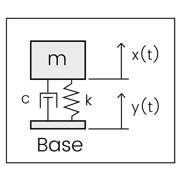
The mass-spring-damper system above is governed by the following differential equation:

$$ mddot{x} + cdot{x} + kx = cdot{y} + ky $$

This result can be derived with some Physics 101 knowledge by building a free body diagram and substituting the forces into Newton’s Second Law of Motion equation. Note that (c) represents the damper coefficient, and (k) represents the spring coefficient. If differential equations aren’t your thing, the spring resistance changes with position of the mass/base while the damper resistance changes with velocity of the mass/base.

For this system, there are some other important equations and concepts that will become relevant. I won’t go into their derivation, but you can find a fairly thorough example here.

Undamped Natural Frequency, (omega_n)

This is the frequency at which the system will vibrate when disturbed if there is no damping. It can be calculated by the simple equation:

$$ omega_n = sqrt{frac{k}{m}} $$

Damped Natural Frequency, (omega_d)

This is the frequency at which the system will actually vibrate when disturbed.

$$ omega_d = omega_n sqrt{1 – zeta^2} $$

where (zeta) is defined as the damping ratio, and is defined by the equation:

$$ zeta = frac{c}{2momega_n} $$

Solving these equations

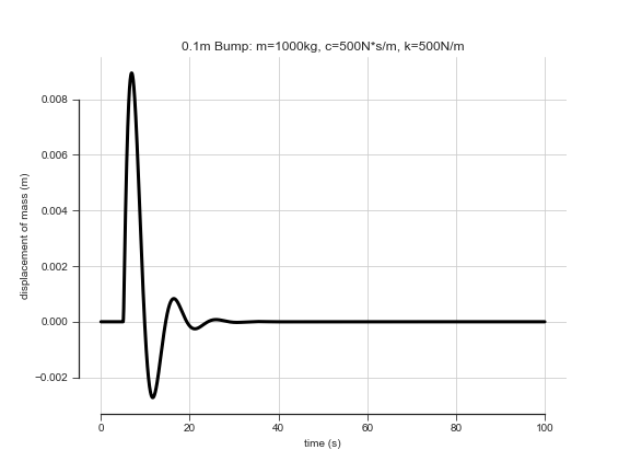
There are many computational solvers for Ordinary Differential Equations. In this case, it was easy to reach for SciPy. Using the SciPy solver, for a single tuple of (m), (c), (k), the position of the mass over time when a car goes over a bump with a height (y=0.1m), looks like:

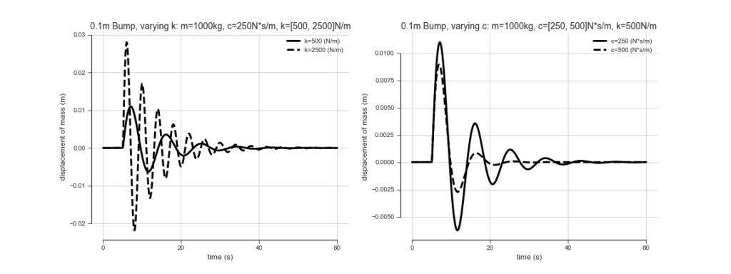
In addition, as (k)/(c) are varied, you can see that the frequency of oscillation and decay rate change respectively.

Designing an Automotive Suspension

Automotive engineer, Pat, works for a hot new automotive company, ALSET. Pat is helping to design a new luxury sedan that will turn the industry upside down because it will be built with “Digital Twin Technology.” Pat is in charge of the suspension, and is under a time crunch, choosing the simplified model shown above.

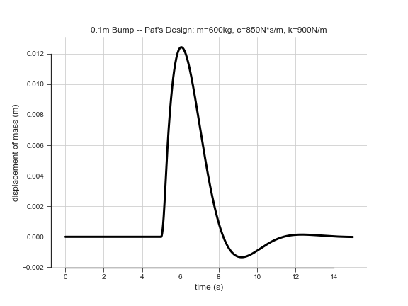
Because Pat is working on a luxury sedan, Pat will design the suspension to be comfortable. This means that the design will target roughly (1Hz) oscillation frequency, which will decay to less than 5% of max displacement after 5 seconds. The target mass of the car is fixed at (2400kg) and is evenly distributed between all four wheels. This means each mass-spring-damper system will have a mass of (frac{2400kg}{4} = 600kg). Using the given constraints and the modeling equations above, Pat can find a (k) and (c) that will theoretically yield the following curve when the car drives over a (0.1m) bump:

Pat’s designs are put into the prototype, and everyone loves the way the car rides, but this is just step one of the digital twin process.

Sensing Suspension Behavior

Though Pat has done some nice digital modeling, the boss, Nole, is not yet satisfied. A core part of the digital twin concept is tracking the real-world item through its lifetime, and making constant comparisons between it and the digital model.

To make this possible, Pat mounts an accelerometer on each corner of the chassis, and hooks each one into the on-board control module. This module periodically streams data from the suspension and other critical systems to ALSET servers. Though Pat will be tracking acceleration, as opposed to position, it is possible to calculate position as the second integral of acceleration. Though this can get complicated when there are multiple axes of motion, it is relatively simple and reliable in one dimension. It should also be noted that the vibrational characteristics of the system are identical whether you are observing an acceleration graph or a position graph.

Before the design is set for production, the prototype car drives on a test track while streaming data from all the on-board sensors. Pat pays special attention to the “bumps” portion of the course. This portion sends the car over (0.1m), (0.2m), and (0.3m) bumps, which yields the following graph:

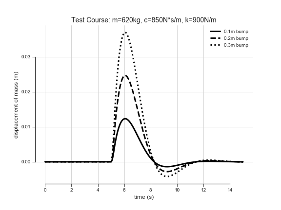
Because of design changes in other parts of the sedan, the results don’t match Pat’s model exactly. However, it is easy to use these data to infer a new model, so Pat does just that.

After a test production run, 10 cars are randomly sampled to drive on the test track, and their results are all nearly identical to the prototype.

Leveraging Twin Data Right Away

Five thousand cars are sold the first week after launch, and Pat receives suspension data from each of them. By running a large map-reduce job, Pat obtains the frequencies and damping ratios from many “bump” events for each of the 5,000 cars and plots the distributions:

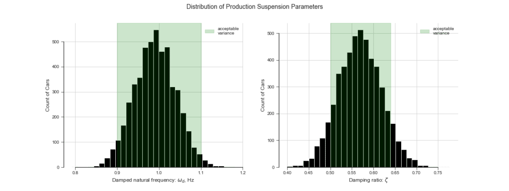
At this scale, it can be seen that there is more variance than desired for some of the key performance constraints. There have been no customer complaints, but Pat notifies the production team, and the team puts measures in place to assemble the suspension with greater consistency.

Big Paybacks in the Long Run

A year later, some warranty claims begin trickling in. The main complaint is unwanted shaking/vibration. Pat looks at the data from some of the claims, and sees something like this:

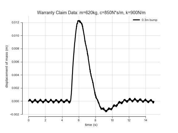
As a seasoned suspension expert, Pat knows this extra vibration is probably due to a worn bushing or failure of some other rubber component, and alerts the repair technicians. Most repair technicians find that the upper spring seat is severely worn to the point of failure. The production team reports that the OEM supplier for this part has been flaky, and the due to high production demands, they have had to work with several backup suppliers and were unable to track which version of the part went into each car.

Total failure of this part could cause unpredictable vehicle handling, and Nole is on the verge of issuing a massive recall. This has huge financial implications, because replacing the part requires removing most of the suspension, and is very time consuming. Before the recall, Nole puts all hands toward finding a better solution.

While combing through the data of all the warranty claims, Pat realizes that there were signs of the imminent failure long before the customers reported a problem. Though the team can’t directly identify cars with faulty parts, they can monitor the entire fleet and determine if something has gone awry.

Nole is relieved, and Pat is a hero. Pat works with an ALSET data scientist to finalize a predictive model, which works by comparing the real-world data with the theoretical suspension model. This leads to car owners being selectively notified of the pending part failure as needed, saving the company millions.

Wrapping Up

Pat’s story has shown us a (simplified) real-world example of digital twin technology. In this example, a failure prediction algorithm was implemented reactively. But anomaly detection for failure prediction can be put in place preemptively if the use case warrants it. The key is that neither are possible if you aren’t collecting data or do not have a computational model of the system (whether physics-based or learned via machine learning).

Though digital twin technology does have origins in rocket science, it’s not that hard to understand, and even a simple model can be valuable. Of course, like anything, as the system gets more complex, or the requirements for model precision get higher, it can become a very difficult problem.

At Very, our data scientists and engineers are familiar with these problems and can work independently or with your engineers to develop a robust, scalable, digital twin solution.